Data Cleaning in Excel

“I always say that the solution to any problem lies in analyzing the problem itself.”

Let’s see the story :-

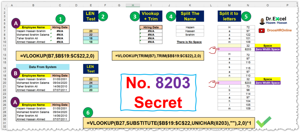
The request says: I want to know the hiring dates for employees in Range A?
Well, the question is easy: I used VLOOKUP, which is one of the most popular search formulas in Excel, and I searched in Range B because it contains the name and date.

This is the equation:

=VLOOKUP(B6;$B$18:$C$21;2;0)

But unfortunately, the result of the equation was #NA.
How come when the names are the same in range B?
There might be extra spaces. So, I used the LEN formula to make sure…and indeed I found that the number of characters for the names in range B is greater than the names in range A.
I used the TRIM formula to get rid of all the extra spaces…and applied it on the search value (the names in range A) and also on all the data in range B.

This is the equation:

=VLOOKUP(TRIM(B6);TRIM($B$18:$C$21);2;0)

But unfortunately, the result of the equation was still #NA? Let’s try to split the name into a set of names, maybe an empty cell will show up or understand what the problem is.
I applied the TEXTSPLIT formula on the names in Range B:

=TEXTSPLIT(B18;;" ")

But no empty cells were displayed. My last option is to split each character by itself.

This is the equation:

=MID(B18;SEQUENCE(LEN(B18));1)

And from here I started to discover the problem…
I found two spaces between each name, there are two spaces…how?
If they are actually spaces, they would have been removed when using the TRIM formula.
I used the UNICODE formula to know what’s happening…

=UNICODE(M5#) 

The number of the real space as a result of the UNICODE formula is 32, and it appeared…but the second space appeared with a different number: it’s 8203…? What’s this?
After researching, I found that it’s called a zero-width space: simply, we can consider it imaginary spaces, but they exist. So now, what’s the solution to get rid of them? Replace them.
This was the equation:

=VLOOKUP(B26;SUBSTITUTE($B$18:$C$21;UNICHAR(8203);"");2;0)*1

I used the SUBSTITUTE formula for replacement, and used UNICHAR. Here, I tell Excel exactly to find out what the number 8203 means using the UNICHAR formula and completely remove the result from the cell. Then, I multiplied it by 1 to activate the number and convert it to a date format.

The File: